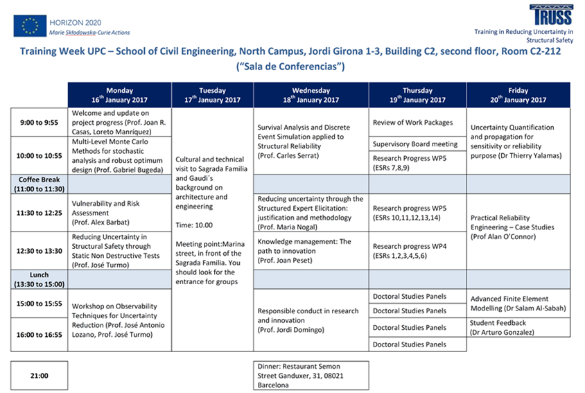


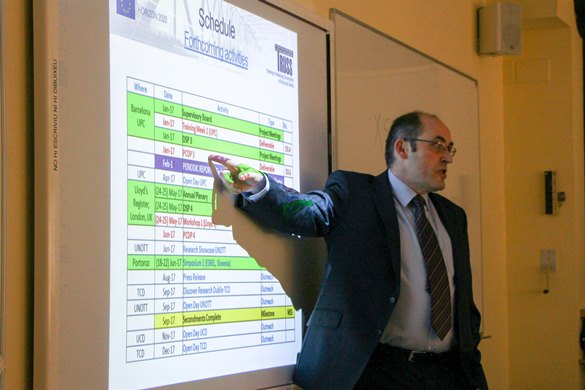


TRUSS second training week was held in Barcelona at Universitat Politècnica de Catalunya from Monday 16th to Friday 20th January 2017. The schedule for the week can be found at the bottom of this page. The questions addressed in each module are described in the expandable toggles below.
To give ESRs an update on the progress of the project and forthcoming activities.
Description
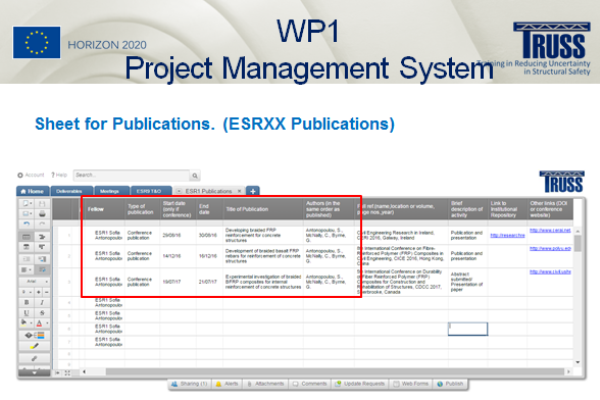
TRUSS achievements and progress in all Work Packages are presented to the ESRs. ESRs are reminded on the importance of keeping the info on training, research and dissemination in their individual sheets of the Project Management System (PMS) complete, accurate and up to date. They are informed of changes introduced in the individual sheets to facilitate consistency in the data gathered from the ESRs. ESRs are explained how the information required in the PMS is transferred into the reports for the European Commission.
-

- Loreto Manriquez, TRUSS Project Manager

-

- Update on Project Progress
Core Research Modules
Core research modules build on modules provided at the 1st training week in UNOTT where basics of “Methods of Safety Quantification”, “Reliability Analysis” and “Life Cycle Assessment” were covered. Four reliability topics with advanced statistical concepts are the focus of the 2nd training week: “Vulnerability and risk assessment”, “Uncertainty Quantification and Propagation for Sensitivity or Reliability Purpose”, “Practical Reliability Engineering – Case Studies” and “Survival Analysis and Discrete Event Simulation applied to Structural Reliability”.
Objective
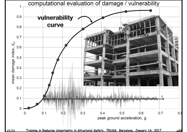
Vulnerability and risk assessment is discussed using the context of the susceptibility of buildings to suffer seismic damage as basis. The seismic vulnerability and risk of buildings and urban areas is treated from intuition to probabilistic evaluation.
Description
Case studies include the Computer Centre of the Telecommunication Ministry in Bucharest (Romania) in 1977, Le Corbusier, Domino House in 1915, and structural failures during the earthquake in Lorca (Spain) on 11th May 2011. Risk is a probabilistic concept => the use of probabilistic risk assessment models is not optional. Damage can be assessed by plotting a vulnerability curve with mean damage index in the vertical axis and peak ground acceleration in the horizontal axis. For this purpose, structural properties such as yielding strength of steel are treated as random variables and modelled via cumulative density functions. The seismic demand is modelled via spectral acceleration (g) versus period (s) graphs. Mean vulnerability curves (DI-PGA) and associated uncertainties (standard deviation of DI-PGA) can then be built. Concepts such as the seismic intensity exceedance rate, intensity parameter, return period of the earthquake, hazard curve (exceedance rate of the intensity versus seismic intensity), average annual loss are introduced.
Vulnerability functions, hazard curves and loss related to long return periods are reviewed for the case of an earthquake in Lorca. The concept of mean damage ratio for a single hazard scenario is explained. Then, it is shown how simulated damage resembles the observed damage in % of buildings for Lorca in the categories: no damage, habitable, non-structural damage (usable after reparation), structural damage (currently not usable) and demolition order (severe structural damage). It is concluded that observed and simulated damage results have the same order of magnitude and huge uncertainties.
-

- Prof Alex Barbat, Universitat Politècnica de Catalunya

-

- Vulnerability and Risk Assessment
The objective is to introduce the general methodology for uncertainty propagation, the methods for sensitivity and reliability analysis, their application to a civil engineering context and the software tools available to carry out this analysis.
Description
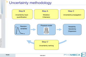
Three steps are distinguished within uncertainty methodology:
- Step A is the physical model, which include the mathematical modelling of the physic (analytical model, numerical model –FEM- and response –surrogate- model), quantity of interest determination and criteria (deterministic –max or min-, probabilistic –dispersion, or probability to exceed a threshold-, or no criteria –ranking of input parameter-).
- Step B is the uncertainty model, which deals with the experimental data available (probability density estimation, statistical validation tests, correlation estimations, etc.) or no specific data available (expert based probabilistic definition for each parameter).
- Step C is the uncertainty propagation that transforms the physical reality into a reliability analysis (probability of failure) following Step A (model and failure scenario) and Step B (probabilistic model).Monte Carlo simulation, Quadrature methods and Quadratic Cumul methods are discussed as methods of uncertainty propagation for sensitivity analysis. Monte Carlo method is the most natural and it consists of generating a sample of the input, computing the output for each set of input parameters and evaluating statistical moments on the output sample. Then a descriptive analysis or inferential analysis can be performed on the output. The inconvenience of Monte Carlo can be the requirements in computational resources (many calls to the physical model). The Quadrature method is a numerical problem that solves statistical moments under integral form by means of a discrete sum. Statistical moments can be obtained with a relatively small number of calls to the physical model for a limited number of input parameters. The Quadratic Cumul approximation is based on Taylor series expansion. It only requires the model response and partial derivatives of the response at the mean, but it is impossible to quantify the error due to the approximation of the model.The use of Monte Carlo simulation, approximation methods (FORM, SORM) and advanced simulation methods (importance sampling, directional sampling, subset sampling, and metamodeling) as methods of uncertainty propagation for reliability assessment are also reviewed. Finally, a practical demonstration is carried out using the graphical capabilities of Phimeca software.
-
- Dr Thierry Yalamas, Phimeca Engineering

-
- Uncertainty Quantification and Propagation for Sensitivity or Reliability Purpose

Practical Reliability Engineering – Case Studies, by Prof Alan O’Connor, from Trinity College Dublin
To demonstrate the significant cost savings via probabilistic methods that can prevent a structure from unnecessary replacement/rehabilitation/repairs by demonstrating the required structural safety is met.
Description
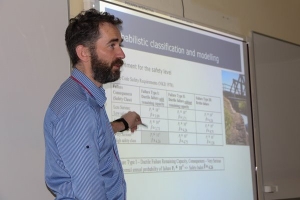
The formal guidelines for probabilistic-based assessment of highway structures by the Danish Roads Directorate is presented as reference. A deterministic approach should be applied first. Probabilistic assessment is recommended only if the deterministic approach establishes that repair, rehabilitation or replacement are needed. Probabilistic assessment involves statistical modelling of load and resistance parameters obtained through on-site measurements and from as-built drawings. Comparison of the probability of failure with that specified by legal requirements is used to validate the safety of the structure. The requirements at the ultimate limit state (i.e., Probability of failure or safety index, ) are specified with reference to failure types and failure consequences:
- Failure Type I – Ductile failure with remaining capacity
- Failure Type II – Ductile failure without remaining capacity
- Failure Type III – Brittle failureIn addition to determination of the value of β, a sensitivity analysis should be performed to determine the sensitivity of β to variations in the parameters describing the stochastic variables modelled in the analysis. The latter allows identifying how small changes in the mean and standard deviations of the random variables affect the safety index.
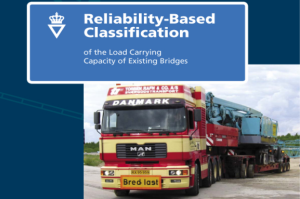
The presentations goes over a number of Danish and Swedish case studies where probabilistic methods have been employed. Results of deterministic results are compared to results of probability-based assessment for 11 bridges, with a total saving in costs of €40,4 million. The probability-based assessment of the Storstroem bridge (Denmark) and the Bergeforsen railway bridge (Sweden) are analysed in detail. While the former is a 3.2 km long bridge exposed to a marine environment with serious deterioration on both the concrete and the reinforcement, the latter is a 168 m single track bridge. Finally, costs of consultant fee, contractor fee, project management and total cost are compared for the three phases of the project:
- Deterministic assessment;
- Advanced deterministic assessment incorporating updated structural models and rain flow analysis for fatigue analysis, and
- Probability based assessment performed at critical locations determined in phase (2).
From the examples provided in this lecture, it is clear that the cost savings resulting from probabilistic assessment have been substantial and that the uncertainty on future maintenance needs have been significantly reduced thereby making overall long-term budgets more accurate and facilitating optimisation of available resources.
-
- Prof Alan O’Connor, Trinity College Dublin

-
- Practical Reliability Engineering – Case Studies

Objective
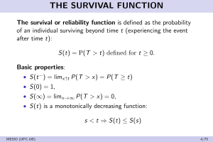
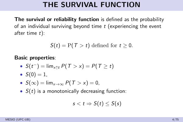
To review basic concepts on survival function, distribution function probability function, hazard function, cumulative hazard function and mean residual lifetime. Focus is placed upon most common parametric models such as Exponential, Weibull, Lognormal and Gamma models. Censoring, likelihood function, truncation and competing risks are also covered.
Description
The survival or reliability function is defined as the probability of an individual surviving beyond time t. The distribution function is defined as the probability of an individual dies before time t. Types of failures:
- Increasing hazard function: Populations with a natural aging or wear. The distribution is called IFR (Increasing Failure Rate);
- Constant hazard function: Populations with no aging. The resulting distribution is the exponential;
- Decreasing hazard function: Populations with a very early likelihood of failure. Individuals get stronger with time. For example, some electronic components in solid state or patients after a transplant. The distribution is called DFR (Decreasing Failure Rate). We find a DFR pattern at the beginning of life of any living being;
- Hazard function with bathtub shape: decreasing at the beginning, constant during a long period of time and increasing at the end of life. Appropriated as a model for populations that are followed from birth. A lot of mortality data follows this kind of curves since at the beginning death are due to childhood disease, later on the failure rate keeps stable and finally we get an increasing failure due to the population aging;
- Hazard function with hump shape: it grows at the beginning and decreases after a period of time. Appropriated as a survival model after surgery since at the beginning there is a high risk of death due to infections and possible hemorrhages, and it decreases as the patient recovers.
In literature about failure times, some parametric models have been used repeatedly. The exponential or Weibull models, for example, are commonly used due to the simplified way that probabilities of distribution tails are expressed, and thus the simplicity of the survival and the hazard function. The lognormal and gamma models, although being less convenient due to computational difficulties, are also often applied. The most commonly used models in survival are Exponential, Weibull, Log-normal, Gamma, Log-logistic and Gompertz. In order to decide if any distribution families that we have studied is appropriated for our problem and our data, we can take into account the following points:
- its technical convenience to the statistical inference,
- the reasonable simplicity of the expressions of its survival or hazard function,
- the good behaviour of the hazard function,
- the value of the coefficient of variation and its analysis with respect to the value 1 as an indicator of exponentiality,
- the representation of the asymmetry taking into account that is equal to 2 in an exponential model, 0 in a normal model and 2/k in a gamma family,
- the behaviour of the survival function for large values of time, and
- the possible connections with a failure model.On the other hand, it is important to realize that in some cases we will not have enough data to validate the chosen law. In that cases it is very important the behaviour of the model for early values of time – for example, in industrial applications when studying guarantee periods-, and for large values of time – in many medical applications we will be more interested in the right tail of the distribution, corresponding to large survival times-.
Data is collected within a time window. Events occurring outside this time window are not observed. Individual times-to-event can be observed leading to an exact observation or not observed leading to a censored observation. We refer to censoring when we only know that the time to event has occurred in a certain interval of time. Censored data can be right-censored (Type I, Type II, Random), left-censored, interval-censored and doubly-censored. The likelihood function is written as the product of the contribution of each individual. The effect of the truncation’s condition is to filter the presence of certain individuals in such a way that the investigator are not aware of their existence. Hence, whatever inference is conditioned to that condition:
- It can be to the left when only individuals of a certain age enter the study (These are known as delayed entries),
- It can be to the right when only those individuals who have had the event are observed (That is, only those patients that fail are included in the study. For example, in a study about mortality which is only based on death certificates).
Sometimes individuals are at risk of other events which don’t allow to observe the event of interest: - Failures due to other causes (competing risks analysis) (i.e., death due to causes which are different from the one we are interested in, or Secondary failure causing inactivity of a machine);
- Survival is modelled via the cause-specific hazard function. A few examples are provided.
-

- Prof Carles Serrat, Universitat Politècnica de Catalunya

-
- Survival Analysis and Discrete Event Simulation applied to Structural Reliability
Specialist Research Modules
A module on “Advanced Finite Element Modelling” explains how to model a structure using finite elements and it serves to complement specialist modules on load and material modelling delivered in UNOTT during the 1st week. While structural health monitoring methods based on dynamic measurements and fault diagnostic methods to characterize damage or structural parameters were also covered in UNOTT, the following alternative / complementary methods are discussed during the 2nd week: Monte-Carlo (MC), Multi-Level Monte-Carlo (MLMC), Genetic Algorithms (GA), the Observability Method (OM) (applied to non-destructive static tests) and expert elicitation (when data is insufficient and expert judgment is needed).
Objective
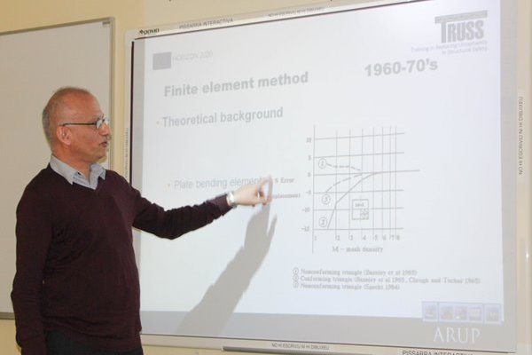
To understand the evolution of finite element modelling from its origins to our time, and the limitations of different types of elements.
Description
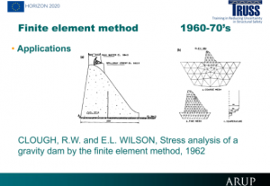
The Finite Element (FE) method is a numerical technique to solve differential equations. These equations date back to the 17th century. There are closed forms solutions for simple differential equations, but most real life applications require more complex Partial Differential Equations, that usually do not have a closed form solution. Numerical solutions to this problem are reviewed historically.
- In the 1920-40’s: Finite difference, lattice of 1D bars, model 3D, square elements, variational forms, flexibility and stiffness, energy principle for matrix methods, the triangular plate element.
- In the 1950’s: the birth of finite element modelling, matrix analysis software, the IBM computer and Fortran. In the 1960’s: isoparametric formulation and applications.
- In the 1960’s-70’s: non-linear elements (geometric, material), plate bending element (Kirchhoff-Germain), conforming elements (2nd order diff. equation – C0 element, 4th order diff. eqn – C1 element), high order 3D elements, commercial software, mathematical foundation and the arc-length method,
- In the 1980-90’s: fluid mechanics, wide applications due to integration of CAD/CAE (automated mesh generation), graphical display of analysis results and powerful and low-cost computers and equation solver (Gauss-Jordan, banded, skyline, sparse).
- In the 2000’s: design optimization, nonlinear analysis, better CAD/CAE integration, parallel processing, more GUI, more integrated analysis/design environment, open source FE packages.
Other topics covered included:
- Element types: point, line, area (plane stress-strain, shell), volume (brick).
- Advanced analysis: Multiphysics (stress analysis, dynamics, heat transfer, fluid flow, convection-diffusion, electromagnetism), fire, topology optimisation, parametric analysis-design-drafting, adaptive mesh refinement, more on material constitutive relations, infinite elements, extended elements, finite volume method, boundary element method, mesh-free methods, etc.
-

- Dr Salam Al-Sabah, Ove ARUP and Partners, Ireland
-
- Advanced Finite Element Modelling

To gather an understanding on how to apply Monte-Carlo (MC) methods, Multi-Level Monte Carlo (MLMC) and Genetic Algorithms (GA) to reduce uncertainty.
Description
Traditional design optimization tools are based on deterministic analysis of each design assuming that the values of all the parameters of the problem definition are well known and fixed. Reality is not like that and there are many parameters with uncertainties in their values. Typically, in solid mechanics real problems there are uncertainties in the geometry, the mechanical properties, the loading conditions, etc. In aeronautics, typical uncertainties affect the Mach number, the angle of attack and also the geometry. Parameters with uncertainties are normally characterised through a probabilistic density function. When a deterministic optimal design is used under off design conditions its performance can decrease a lot unless robustness be introduced in the design process.
Analysis with uncertainties is an important aspect for Robust Design. Methods for analysis with uncertainties can be classified within three categories:
- Statistical methods (multi-point/DOE, Monte-Carlo, Multi-Level MC),
- Intrusive methods (Polynomical Chaos method, Perturbation method, Stochastic Galerkin, Fuzzy FE method) and
- Non-intrusive methods (Probabilistic collocation, Stochastic collocation).
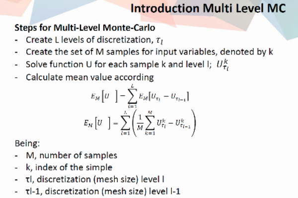
MC is an easy to implement method that generates sampling cases based on the probability density function of each parameter with uncertainties. MC needs a big number of sampling points for a good statistical representation of the stochastic solution (especially big if the number of parameters with uncertainties is big), and a good level of resolution of each deterministic analysis which makes it expensive.
MLMC combines a big number of analysis with a low level of resolution with a small number of analysis with a high level of resolution making the total cost much lower than with classical MC. MLMC is cheaper than MC, providing a better accuracy in mean and variance values. Any kind of discretization is possible with MLMC, mesh is the most relevant.
GA are metaheuristic multi-purpose and random algorithms. Although slower compared to gradient based, they enable to overcome unknown behaviour of the objective functions (discontinuities, non-derivability). GA are always associated to a higher computational cost, compared to other optimization methods. Black box strategy works perfectly well and simplifies the task.
-
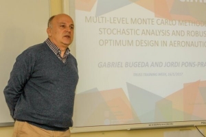
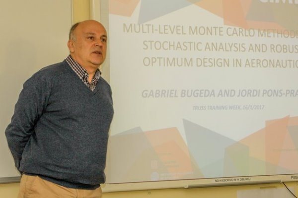
- Prof Gabriel Bugeda, Universitat Politècnica de Catalunya
-

- Multi-Level Montecarlo Methods for Stochastic Analysis and Robust Optimum Design
To bring awareness on the potential of the Observability Method (OM) for structural system identification purposes.
Description
OM is the first efficient method to solve systems of monomial-ratio equations. A subset of variables is observable when the system of equations implies a unique solution for this subset, even though the remaining variables remain undetermined. The applicability of OM is demonstrated for the case of measurements obtained from a controlled static test. Here, the stiffness matrix multiplied by the displacements leads to the forces applied on the structure. In these system of equations, there are known and unknown variables. The following issues are faced:
- Non-linear products of coupled variables appear in these multiplications (linearization),
- target unknowns (i.e., stiffness) is coupled with deflections (decoupling process), and
- observed information not considered (Recursive process).
The OM is a parametric approach to deal with these issues. The minimal measurement set can be established via observability trees. Errors increase at the proximities of zones with zero curvature. OM combines a symbolical and a numerical approach that allow obtaining parametric equations of the estimates. The method is shown to be computationally very efficient.
-

- Prof Jose Turmo, Universitat Politècnica de Catalunya

-
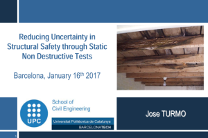
- Reducing Uncertainty in Structural Safety through Static Non-Destructive Tests

The aims of this workshop are understanding: (a) the differences between the direct and the inverse analysis of the stiffness matrix method, (b) how the observability technique is applied, (c) the concept of observability trees and flow, (d) structural system identification of the structure both symbolically and numerically, and (e) future applications on your research field.
Description
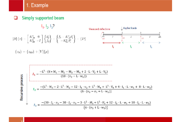
Two examples are carried out to demonstrate how the observability technique can be implemented using Matlab. First, a simply supported beam is discretized into three elements. Global stiffness matrix is assembled, deflections to known applied loads are given, and the inertias of these three beams are sought by the observability method. The symbolical analysis and recursive process are discussed.
The second example is a two-span bridge, a 2D model with 9 nodes and 8 beam elements. The individual stiffness of all beams and boundary conditions are unkowns. Vertical and horizontal loads are applied, and horizontal and vertical displacements and rotations are measured at certain nodes. There are coupled flexural stiffnesses and couple axial stifnesss. The axial observability tree and the flexural observability tree are employed to obtain all stiffnesses in a recursive process. In the workshop, ESRs are taught to use axial and flexural observability trees to define a measurement set that assures an adequate observability of all axial and flexural stiffnesses. Then, a symbolic approach is empoyed to identify the parameters uniquely defined (observable) for the measurements calculated by the preceding point and to obtain their parameteric equations. Finally, the ratio between the estimated and the actual stiffness is assessed for each element for different levels of accuracy in the measurements.
-

- Prof José Antonio Lozano, Escuela Técnica Superior de Ingenieros de Caminos, Canales y Puertos de la Universidad de Castilla-La Mancha

-

- Workshop on Observability Techniques for Uncertainty Reduction
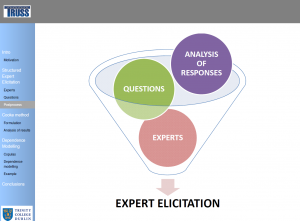
To introduce Expert Elicitation, or the process of synthesis of subjective judgements of experts on a subject where there is uncertainty due to insufficient data because of physical constraints or lack or resources, and “Structured” Expert Elicitation, or the process based on structured protocols to reduce potential sources of bias and error among experts.
Description
The analysis of uncertainty can be addressed under other perspective beyond the frequentist-based probability. Marginal and joint distributions which are expensive or difficult to be measured can be known through the structured expert elicitation. What can we obtain from the experts? Fuzzy set theory (i.e, ranges for cost and damage level), Semi-Quantitative methods (i.e., ranks for model parameters and risk factors, scoring of the relative importance of factors in a scenario) and Quantitative methods (quantitative estimates, uncertainty distributions, dependence modelling) are reviewed.
Delphi method is a behavioural method that looks for the consensus among experts, who are typically encouraged to interact and share their assessments. Cooke’s method is mathematical method that deals with individual assessments, and combine them mathematically after their elicitation to yield more accurate results. The Cooke’s method for the uncertainty distribution of the random variables is well-developed and widely used. In Cooke’s method, calibration measures the statistical likelihood that a set of experimental results statistically correspond with the expert’s assessments. Assuming as a null hypothesis that the inter-quantile interval containing the true value for each variable is drawn independently from the probability vector p, the expert’s assessment can be treated as a statistical hypothesis, and the p-value can be used as a calibration score. Informativeness considers how concentrated a distribution is. To measure it, the density of the sample distribution provided by the expert e for the quantity i is compared against a background probability density (usually uniform or log uniform distribution) over the extended intrinsic range. The Decision Maker or combination of experts’ assessment is carried out by the summation of the experts’ assessments of the variables of interest, weighted according the scores obtained.
Dependence modelling and the high potential with a number of applications are explored. Copula is a multivariate probability distribution for which the marginal probability distribution of each variable is uniform. The multivariate Gaussian copula is discussed. In Bayesian networks, each node is associated with a continuous arbitrary invertible distribution function and each parent-child influence is represented as a (conditional) one parameter copula, parameterised in terms of the (conditional) rank correlation. When all copulas in the assignment of a Non-Parametric Bayesian Network correspond to the bivariate normal copula, then a multivariate Gaussian copula with correlation matrix is obtained. D-calibration measures the distance between a “seed” correlation matrix and the correlation matrix obtained based on experts’ opinion. An example to assess the vulnerability of a traffic system through numerical indicators is carried out.
-

- Dr Maria Nogal, Trinity College Dublin

-
- Reducing Uncertainty through the structured Expert Elicitation: Justification and Methodology

Communication/Transferable Skills Modules
The module “Knowledge Management: the Path to Innovation” is provided by the Head of the relevant Department in a TRUSS industrial partner. This module builds on the basics for project management that were provided in the module “Planning your Research” at the 1st training week. ESRs also become aware of a variety of important moral and social values promoted by research via the module “Responsible Conduct in Research and Innovation”.
To share with ESRs the significance of Knowledge Management and Innovation, and the experience of working in a specialised Department on this topic.
Description
The Head of Knowledge Management and Innovation Department introduces the topics covered in a research management position. The areas of activity of COMSA in Infrastructure and Engineering, Services and Technology and Concessions and Renewable Energy are explained. Subsidiary companies also make a significant contribution to construction and maintenance works at specific countries. The focus is then placed upon railway infrastructure, which has been the main speciality of the company form its foundation. The service goes from the initial study and project design to the construction and maintenance of railway infrastructures and superstructures, metros and trams, including their operation. In the Department of Knowledge Management and Innovation, clients/suppliers, academia and business units expertise guide the technological challenges to address. There are a number of key activities within the Department:
- acquiring know-how (benefiting from work site experience). The strong collaboration between the technical department and the work site permits and easy and quick transfer of knowledge;
- tools (technical procedures and IT tools). All the know-how acquired form the work site has to be well managed and stored in order to be applied in the next projects. A great way to gather together this information is creating technical procedures, where not only a description of the works can be found but also output and construction cost rates. Data Bases can offer a great improvement in information accessibility, which contributes to make easier the access and transfer of information;
- Technical support. The Technical Dept. gives support to the work site in each step of the project (from the study/ tender process of the project until the reception of the work site). All the innovation and know-how of the Technical Dept. are conveniently applied in order to improve economically and technically the projects;
- R&D strategy. Innovation represents nowadays one of the top drivers of growth of a company. Improving construction methods by applying advanced technology enable not only to reduce cost and execution time of the work site, but also helps to reinforce the leader position of the company;
- Lean construction. The goal is to improve the efficiency of the construction works by eliminating the “waste” (activities with no added value for the client). Building Information Modelling (BIM) is also discussed and a number of ongoing and recently completed projects are reviewed.
-
- Prof Joan Peset, COMSA
-

- Knowledge Management: The Path to Innovation
-

To facilitate the pillars for a responsible conduct in research.
Description
Responsible conduct is not easy to define. It is about ethics … about common accepted rules or behaviour. There is not a single “best way” to undertake research, there are specific ways in different scientific fields. Accepted practices vary from discipline to discipline and even from lab to lab or group to group. Scientific/Professional societies or communities publish codes of conduct. Misconduct is fabrication, falsification or plagiarism in proposing, performing or reviewing research, or in reporting research results. Research misconduct does not include honest error or differences of opinion. Four responsible conduct pillars can be distinguished:
- Government Regulations. Definition of what is and is not allowed; penalties;
- Professional Codes. List of principles; general statements; set a minimum standard; do not imply that all other behaviours are accepted;
- Institutional Policies. Promotion of good practices; establish definitions for misconduct in research; define procedures for reporting and investigating misconduct; provide protection for whistle-blowers and persons accused of misconduct; Researchers and research institutions bear the primary responsibility for reporting and investigating misconduct; the position that research is a profession and should regulate its own conduct, is strongly supported by most researchers;
- Personal Convictions. Personal ethics. Institutional policies help to establish a suitable framework to avoid misconduct and to deal with it if necessary, but they do not solve the problem. Personal responsibility is the key factor. In general terms, responsible conduct in research is simply good citizenship applied to professional life. A number of topics including shared values (honesty, accuracy, efficiency and objectivity) and misconduct, authorship, plagiarism, peer review, conflicts of interests, mentoring, collaborative research and data management practices are reviewed.
-

- Prof Jordi Domingo, Universitat Politècnica de Catalunya
-

- Responsible Conduct in Research and Innovation

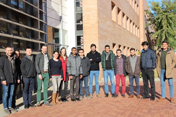
Team Activities
A cultural and technical visit organised by Universitat Politècnica de Catalunya, aimed to form powerful relationships supporting each other’s professional growth.
To give ESRs and supervisors an overview of the constructions works in the Sagrada Familia guided by an architect involved in the task, and also, to learn about his creator Gaudi from an architectural and engineering points of view. To promote team cohesion and networking between ESRs and UPC/TCD supervisors and lecturers in an informal environment.
Description
Actual and planned construction was showed by architect Jaume Serrallonga. He explained how the construction team have based their work on original 3D models and drawings from Gaudi. He explained how the majority of works are prefabricated on a site outside Barcelona due to space restrictions. The construction of the Passion Facade and the dome of the Sacristy of Passion, the roofs and the meaning of their colours, were discussed in detail. Works on the different towers such as the Evangelists, Virgin Mary and Jesus Christ were also described in detail. Building works for the Sagrada Familia are expected to be finished in 9 years.
-

- Jaume Serrallonga, Project Architect

-

- The Sagrada Familia, project and works

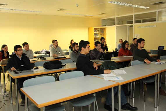
Research Seminars
Objective
To prepare ESRs to present their own work at national and international events via interactive presentations on their individual research projects. Presentations are followed by face-to-face Doctoral Studies Panel (DSP) meetings that allow fellows to get feedback from the consortium for their Research and Personal Career Development Plans (PCDPs).
Description
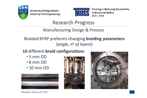
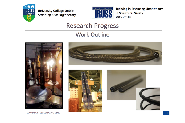
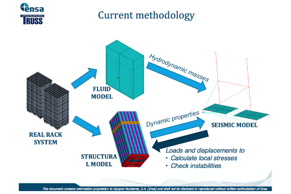
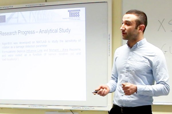
These seminars are confined to TRUSS partners and researchers local to the host venue who wished to attend. ESRs have the opportunity to practise communication skills that were taught at the module on public speaking titled “Presentation Skills” in the 1st training week. Practice makes perfect, however, a proper feedback process is needed, and for that purpose, all presentations in this 2nd training week were fully recorded in video and made available to ESRs internally for self-evaluation and for avoiding mistakes. In this 2nd training week, the theme of each presentation has been around the research progress and plans following their first year with TRUSS. After presentations, each ESR was called on an individual basis for focus meetings with his/her DSP and discussing the PCDP.


ESR Feedback
At the end of the training week, answers to a confidential questionnaire were gathered from fellows to identify those modules found more useful for the project and for their future career and to propose new modules to cover their needs or a follow-up to existing ones in a future training event.
Click the image below to see the schedule